LSTM Stock Prediction
INFO
Time Series, Quantitative Trading, Time Series Model
Overview
LSTM (Long Short-Term Memory), a special type of RNN (Recurrent Neural Network), improves the traditional RNN's issues of gradient vanishing and gradient explosion when handling long sequence data. Proposed by Hochreiter and Schmidhuber in 1997, LSTM has become one of the classic models for processing time series data.

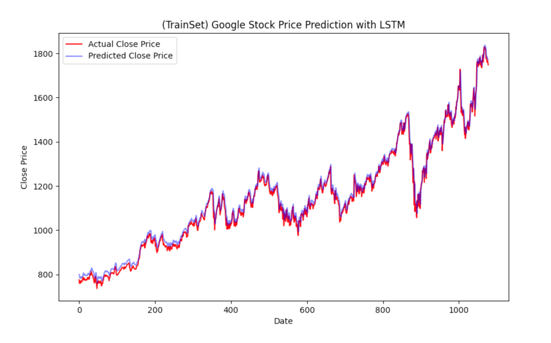
Stock prediction tasks involve predicting the current and future stock price changes based on past data of a stock using AI models. This is also a practical time series task. Here, we use the Google stock price dataset from 2016 to 2021 for training and inference.
Environment Setup
This case study is based on Python>=3.8. Please ensure Python is installed on your computer. Environment dependencies:
pandas
torch
matplotlib
swanlab
scikit-learn
Quick installation command:
pip install pandas torch matplotlib swanlab scikit-learnThis code is tested on torch==2.3.0, pandas==2.0.3, matplotlib==3.8.2, swanlab==0.3.8, scikit-learn==1.3.2
Complete Code
Please download the Google Stock Prediction dataset from Kaggle to the root directory.
import os
import swanlab
import torch
import torch.nn as nn
import torch.optim as optim
from torch.utils.data import DataLoader
import matplotlib.pyplot as plt
from copy import deepcopy as dc
import numpy as np
import pandas as pd
from torch.utils.data import Dataset
from sklearn.preprocessing import MinMaxScaler


class LSTMModel(nn.Module):
    """
    Define the model class
    """
    def __init__(self, input_size=1, hidden_size1=50, hidden_size2=64, fc1_size=32, fc2_size=16, output_size=1):
        super(LSTMModel, self).__init__()
        self.lstm1 = nn.LSTM(input_size, hidden_size1, batch_first=True)
        self.lstm2 = nn.LSTM(hidden_size1, hidden_size2, batch_first=True)
        self.fc1 = nn.Linear(hidden_size2, fc1_size)
        self.fc2 = nn.Linear(fc1_size, fc2_size)
        self.fc3 = nn.Linear(fc2_size, output_size)

    def forward(self, x):
        x, _ = self.lstm1(x)
        x, _ = self.lstm2(x)
        x = self.fc1(x[:, -1, :])
        x = self.fc2(x)
        x = self.fc3(x)
        return x


class TimeSeriesDataset(Dataset):
    """
    Define the dataset class
    """
    def __init__(self, X, y):
        self.X = X
        self.y = y

    def __len__(self):
        return len(self.X)

    def __getitem__(self, i):
        return self.X[i], self.y[i]


def prepare_dataframe_for_lstm(df, n_steps):
    """
    Process the dataset to be suitable for LSTM model
    """
    df = dc(df)
    df['date'] = pd.to_datetime(df['date'])
    df.set_index('date', inplace=True)

    for i in range(1, n_steps+1):
        df[f'close(t-{i})'] = df['close'].shift(i)

    df.dropna(inplace=True)
    return df


def get_dataset(file_path, lookback, split_ratio=0.9):
    """
    Normalize data and split into training and test sets
    """
    data = pd.read_csv(file_path)
    data = data[['date','close']]

    shifted_df_as_np = prepare_dataframe_for_lstm(data, lookback)

    scaler = MinMaxScaler(feature_range=(-1,1))
    shifted_df_as_np = scaler.fit_transform(shifted_df_as_np)

    X = shifted_df_as_np[:, 1:]
    y = shifted_df_as_np[:, 0]

    X = dc(np.flip(X,axis=1))

    # Split into training and test sets
    split_index = int(len(X) * split_ratio)

    X_train = X[:split_index]
    X_test = X[split_index:]

    y_train = y[:split_index]
    y_test = y[split_index:]

    X_train = X_train.reshape((-1, lookback, 1))
    X_test = X_test.reshape((-1, lookback, 1))

    y_train = y_train.reshape((-1, 1))
    y_test = y_test.reshape((-1, 1))

    # Convert to Tensor
    X_train = torch.tensor(X_train).float()
    y_train = torch.tensor(y_train).float()
    X_test = torch.tensor(X_test).float()
    y_test = torch.tensor(y_test).float()

    return scaler, X_train, X_test, y_train, y_test


def train(model, train_loader, optimizer, criterion):
        model.train()
        running_loss = 0
        # Training
        for i, batch in enumerate(train_loader):
            x_batch, y_batch = batch[0].to(device), batch[1].to(device)
            y_pred = model(x_batch)
            loss = criterion(y_pred, y_batch)
            running_loss += loss.item()
            optimizer.zero_grad()
            loss.backward()
            optimizer.step()

        avg_loss_epoch = running_loss / len(train_loader)
        print(f'Epoch: {epoch}, Batch: {i}, Avg. Loss: {avg_loss_epoch}')
        swanlab.log({"train/loss": running_loss}, step=epoch)
        running_loss = 0


def validate(model, test_loader, criterion, epoch):
    model.eval()
    val_loss = 0
    with torch.no_grad():
        for _, batch in enumerate(test_loader):
            x_batch, y_batch = batch[0].to(device), batch[1].to(device)
            y_pred = model(x_batch)
            loss = criterion(y_pred, y_batch)
            val_loss += loss.item()
        avg_val_loss = val_loss / len(test_loader)
        print(f'Epoch: {epoch}, Validation Loss: {avg_val_loss}')
        swanlab.log({"val/loss": avg_val_loss}, step=epoch)


def inverse_transform_and_extract(scaler, data, lookback):
    dummies = np.zeros((data.shape[0], lookback + 1))
    dummies[:, 0] = data.flatten()
    return dc(scaler.inverse_transform(dummies)[:, 0])


def plot_predictions(actual, predicted, title, xlabel='Date', ylabel='Close Price'):
    """
    Plot the final stock price prediction versus the actual values
    """
    plt.figure(figsize=(10, 6))
    plt.plot(actual, color='red', label='Actual Close Price')
    plt.plot(predicted, color='blue', label='Predicted Close Price', alpha=0.5)
    plt.xlabel(xlabel)
    plt.ylabel(ylabel)
    plt.title(title)
    plt.legend()
    return swanlab.Image(plt, caption=title)


def visualize_predictions(train_predictions, val_predictions, scaler, y_train, y_test, lookback):
    train_predictions = inverse_transform_and_extract(scaler, train_predictions, lookback)
    val_predictions = inverse_transform_and_extract(scaler, val_predictions, lookback)
    new_y_train = inverse_transform_and_extract(scaler, y_train, lookback)
    new_y_test = inverse_transform_and_extract(scaler, y_test, lookback)

    plt_image = []
    plt_image.append(plot_predictions(new_y_train, train_predictions, '(TrainSet) Google Stock Price Prediction with LSTM'))
    plt_image.append(plot_predictions(new_y_test, val_predictions, '(TestSet) Google Stock Price Prediction with LSTM'))

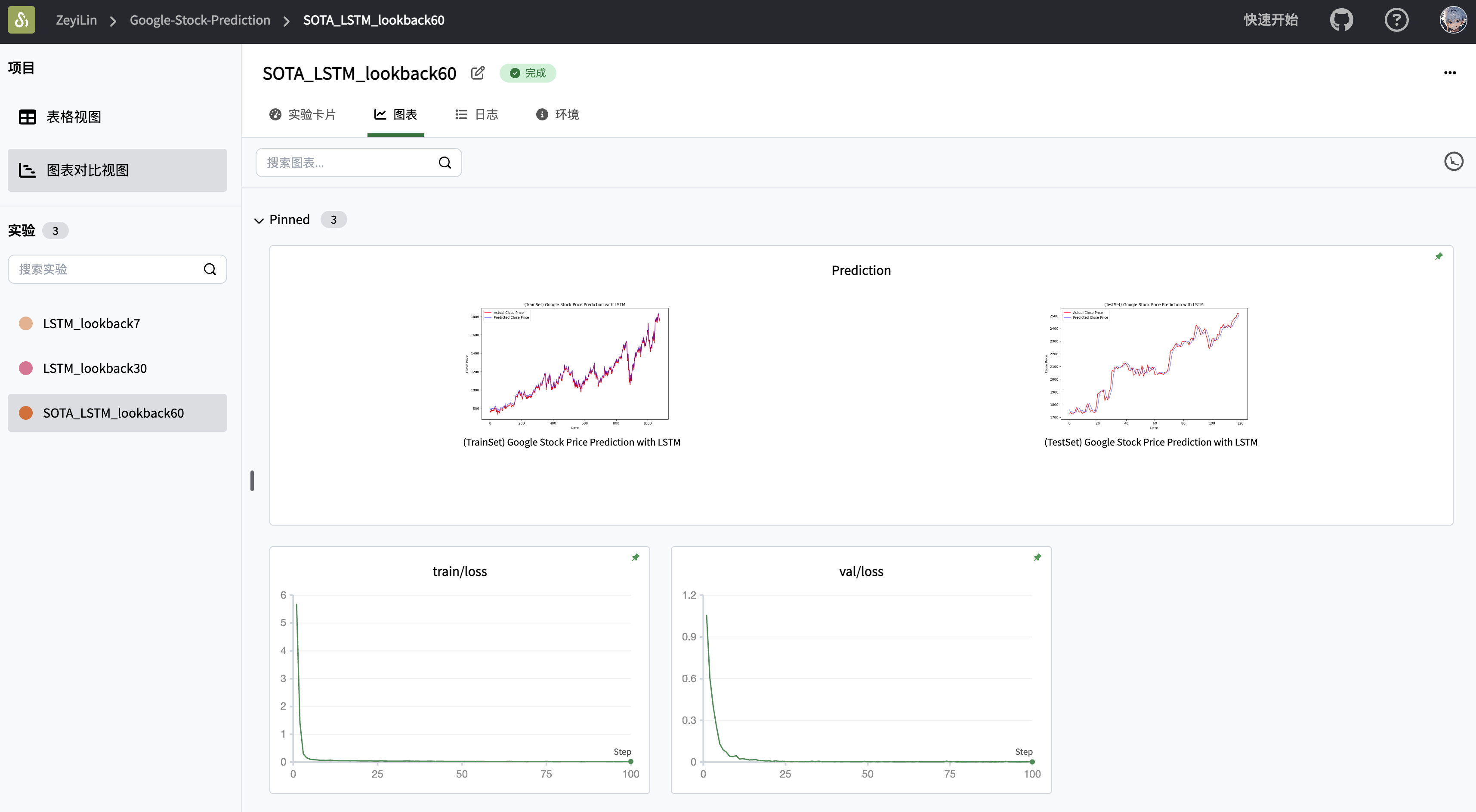
    swanlab.log({"Prediction": plt_image})


if __name__ == '__main__':
    # ------------------- Initialize a SwanLab experiment -------------------
    swanlab.init(
        project='Google-Stock-Prediction',
        experiment_name="LSTM",
        description="Predict the next day's stock price based on the previous 7 days' data",
        config={
            "learning_rate": 1e-3,
            "epochs": 100,
            "batch_size": 32,
            "lookback": 7,
            "spilt_ratio": 0.9,
            "save_path": "./checkpoint",
            "optimizer": "Adam",
            "device": 'cuda' if torch.cuda.is_available() else 'cpu',
        },
    )

    config = swanlab.config
    device = torch.device(config.device)

    # ------------------- Define the dataset -------------------
    scaler, X_train, X_test, y_train, y_test = get_dataset(file_path='./GOOG.csv',
                                                           lookback=config.lookback,
                                                           split_ratio=config.spilt_ratio,)

    train_dataset = TimeSeriesDataset(X_train, y_train)
    test_dataset = TimeSeriesDataset(X_test, y_test)

    train_loader = DataLoader(train_dataset, batch_size=config.batch_size, shuffle=True)
    test_loader = DataLoader(test_dataset, batch_size=config.batch_size, shuffle=False)

    # ------------------- Define the model and hyperparameters -------------------
    model = LSTMModel(input_size=1, output_size=1)

    model = model.to(device)
    optimizer = optim.Adam(model.parameters(), lr=config.learning_rate)
    criterion = nn.MSELoss()

    # ------------------- Training and validation -------------------
    for epoch in range(1, config.epochs+1):
        train(model, train_loader, optimizer, criterion)
        validate(model, test_loader, criterion, epoch)

    # ------------------- Use the best model for inference and generate visualization results -------------------
    with torch.no_grad():
        model.eval()
        train_predictions = model(X_train.to(device)).to('cpu').numpy()
        val_predictions = model(X_test.to(device)).to('cpu').numpy()
        visualize_predictions(train_predictions, val_predictions, scaler, y_train, y_test, config.lookback)

    # ------------------- Save the model -------------------
    model_save_path = os.path.join(config.save_path, 'lstm.pth')
    if not os.path.exists(config.save_path):
        os.makedirs(config.save_path)
    torch.save(model.state_dict(), model_save_path)
Demonstration of Results
