UNet for Medical Image Segmentation

INFO

Computer Vision, Medical Imaging, Image Segmentation

Training Process

UNet is a convolutional neural network (CNN)-based model for medical image segmentation, proposed by Ronneberger et al. in 2015. In this article, we will briefly introduce training a UNet model on a brain tumor medical image segmentation dataset using the PyTorch framework, while monitoring the training process with SwanLab to achieve intelligent localization of lesion areas or organ structures.

• Code: Full code available in Section 5 or on GitHub
• Training Logs: Unet-Medical-Segmentation - SwanLab
• Model: UNet (implemented directly in PyTorch)
• Dataset: brain-tumor-image-dataset-semantic-segmentation - Kaggle
• SwanLab: https://swanlab.cn

1. Environment Setup

The environment setup consists of three steps:

1. Ensure your computer has at least one NVIDIA GPU with CUDA installed.
2. Install Python (version ≥ 3.8) and PyTorch with CUDA support.
3. Install third-party libraries required for UNet fine-tuning using the following commands:

git clone https://github.com/Zeyi-Lin/UNet-Medical.git
cd UNet-Medical
pip install -r requirements.txt

2. Dataset Preparation

This section uses the Brain Tumor Segmentation Dataset, which is specifically designed for medical image segmentation tasks.

Dataset Description: The Brain Tumor Segmentation Dataset is tailored for semantic segmentation in medical imaging, aiming to accurately identify brain tumor regions. It contains binary annotations (tumor/non-tumor) and enables pixel-level classification for fine-grained tumor segmentation. This dataset is suitable for training and evaluating medical image segmentation models, providing automated analysis support for brain tumor diagnosis.

For this task, we will download and extract the dataset for subsequent training.

Download and Extract the Dataset:

python download.py
unzip dataset/Brain_Tumor_Image_DataSet.zip -d dataset/

After completing these steps, you should see the following directory structure:

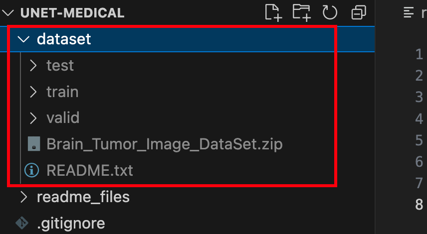
The folder contains training, validation, and test sets with image files (in jpg format) and annotation files (in json format). At this point, the dataset preparation is complete.

Below are some detailed code snippets. If you want to start training immediately, skip to Section 5.

3. Model Implementation

Here, we implement the UNet model in PyTorch (in net.py). The code is shown below:

import torch
import torch.nn as nn

# Define the downsampling block for the U-Net model
class DownBlock(nn.Module):
    def __init__(self, in_channels, out_channels, dropout_prob=0, max_pooling=True):
        super(DownBlock, self).__init__()
        self.conv1 = nn.Conv2d(in_channels, out_channels, 3, padding=1)
        self.conv2 = nn.Conv2d(out_channels, out_channels, 3, padding=1)
        self.relu = nn.ReLU(inplace=True)
        self.maxpool = nn.MaxPool2d(2) if max_pooling else None
        self.dropout = nn.Dropout(dropout_prob) if dropout_prob > 0 else None

    def forward(self, x):
        x = self.relu(self.conv1(x))
        x = self.relu(self.conv2(x))
        if self.dropout:
            x = self.dropout(x)
        skip = x
        if self.maxpool:
            x = self.maxpool(x)
        return x, skip

# Define the upsampling block for the U-Net model
class UpBlock(nn.Module):
    def __init__(self, in_channels, out_channels):
        super(UpBlock, self).__init__()
        self.up = nn.ConvTranspose2d(in_channels, out_channels, kernel_size=2, stride=2)
        self.conv1 = nn.Conv2d(out_channels * 2, out_channels, 3, padding=1)
        self.conv2 = nn.Conv2d(out_channels, out_channels, 3, padding=1)
        self.relu = nn.ReLU(inplace=True)

    def forward(self, x, skip):
        x = self.up(x)
        x = torch.cat([x, skip], dim=1)
        x = self.relu(self.conv1(x))
        x = self.relu(self.conv2(x))
        return x

# Define the complete U-Net model
class UNet(nn.Module):
    def __init__(self, n_channels=3, n_classes=1, n_filters=32):
        super(UNet, self).__init__()

        # Encoder path
        self.down1 = DownBlock(n_channels, n_filters)
        self.down2 = DownBlock(n_filters, n_filters * 2)
        self.down3 = DownBlock(n_filters * 2, n_filters * 4)
        self.down4 = DownBlock(n_filters * 4, n_filters * 8)
        self.down5 = DownBlock(n_filters * 8, n_filters * 16)

        # Bottleneck layer (remove final max-pooling)
        self.bottleneck = DownBlock(n_filters * 16, n_filters * 32, dropout_prob=0.4, max_pooling=False)

        # Decoder path
        self.up1 = UpBlock(n_filters * 32, n_filters * 16)
        self.up2 = UpBlock(n_filters * 16, n_filters * 8)
        self.up3 = UpBlock(n_filters * 8, n_filters * 4)
        self.up4 = UpBlock(n_filters * 4, n_filters * 2)
        self.up5 = UpBlock(n_filters * 2, n_filters)

        # Output layer
        self.outc = nn.Conv2d(n_filters, n_classes, 1)
        self.sigmoid = nn.Sigmoid()

    def forward(self, x):
        # Encoder path
        x1, skip1 = self.down1(x)      # 128
        x2, skip2 = self.down2(x1)     # 64
        x3, skip3 = self.down3(x2)     # 32
        x4, skip4 = self.down4(x3)     # 16
        x5, skip5 = self.down5(x4)     # 8

        # Bottleneck layer
        x6, skip6 = self.bottleneck(x5)  # 8 (no downsampling)

        # Decoder path
        x = self.up1(x6, skip5)    # 16
        x = self.up2(x, skip4)     # 32
        x = self.up3(x, skip3)     # 64
        x = self.up4(x, skip2)     # 128
        x = self.up5(x, skip1)     # 256

        x = self.outc(x)
        x = self.sigmoid(x)
        return x

The model is saved as a pth file, requiring approximately 124 MB.

4. Experiment Tracking with SwanLab

SwanLab is an open-source tool for training experiment tracking. Designed for AI researchers, SwanLab provides training visualization, automatic logging, hyperparameter recording, experiment comparison, and multi-user collaboration. With SwanLab, researchers can identify training issues through intuitive visualizations, compare multiple experiments for inspiration, and share results via online links to facilitate team collaboration.

For this training session, we configure SwanLab with the project name Unet-Medical-Segmentation, experiment name bs32-epoch40, and the following hyperparameters:

swanlab.init(
    project="Unet-Medical-Segmentation",
    experiment_name="bs32-epoch40",
    config={
        "batch_size": 32,
        "learning_rate": 1e-4,
        "num_epochs": 40,
        "device": "cuda" if torch.cuda.is_available() else "cpu",
    },
)

Here, the batch size is 32, the learning rate is 1e-4, and the training runs for 40 epochs.

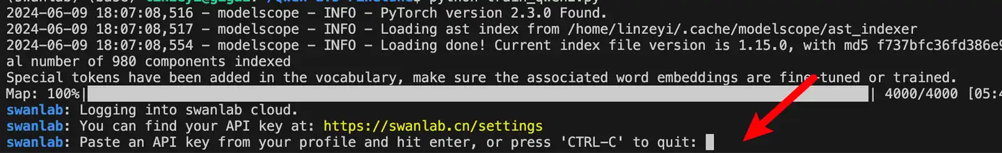
For first-time SwanLab users, register an account on the official website, copy your API Key from the user settings page, and paste it when prompted during training. Subsequent logins will not require this step:

5. Start Training

View the training visualization: Unet-Medical-Segmentation

This section accomplishes the following:

1. Loads the UNet model.
2. Prepares the dataset (training, validation, and test sets) with resizing to (256, 256) and normalization.
3. Uses SwanLab to log training metrics, hyperparameters, and final model outputs.
4. Trains for 40 epochs.
5. Generates final prediction visualizations.

The directory structure before execution should be:

|———— dataset/
|———————— train/
|———————— val/
|———————— test/
|———— readme_files/
|———— train.py
|———— data.py
|———— net.py
|———— download.py
|———— requirements.txt

Full Code

train.py:

import torch
import torch.nn as nn
import torch.optim as optim
import matplotlib.pyplot as plt
from pycocotools.coco import COCO
from torch.utils.data import DataLoader
import torchvision.transforms as transforms
import random
import swanlab
from net import UNet
from data import COCOSegmentationDataset


# Dataset paths
train_dir = './dataset/train'
val_dir = './dataset/valid'
test_dir = './dataset/test'

train_annotation_file = './dataset/train/_annotations.coco.json'
test_annotation_file = './dataset/test/_annotations.coco.json'
val_annotation_file = './dataset/valid/_annotations.coco.json'

# Load COCO datasets
train_coco = COCO(train_annotation_file)
val_coco = COCO(val_annotation_file)
test_coco = COCO(test_annotation_file)

# Loss functions
def dice_loss(pred, target, smooth=1e-6):
    pred_flat = pred.view(-1)
    target_flat = target.view(-1)
    intersection = (pred_flat * target_flat).sum()
    return 1 - ((2. * intersection + smooth) / (pred_flat.sum() + target_flat.sum() + smooth))

def combined_loss(pred, target):
    dice = dice_loss(pred, target)
    bce = nn.BCELoss()(pred, target)
    return 0.6 * dice + 0.4 * bce

# Training function
def train_model(model, train_loader, val_loader, criterion, optimizer, num_epochs, device):
    best_val_loss = float('inf')
    patience = 8
    patience_counter = 0

    for epoch in range(num_epochs):
        model.train()
        train_loss = 0
        train_acc = 0

        for images, masks in train_loader:
            images, masks = images.to(device), masks.to(device)

            optimizer.zero_grad()
            outputs = model(images)
            loss = criterion(outputs, masks)

            loss.backward()
            optimizer.step()

            train_loss += loss.item()
            train_acc += (outputs.round() == masks).float().mean().item()

        train_loss /= len(train_loader)
        train_acc /= len(train_loader)

        # Validation
        model.eval()
        val_loss = 0
        val_acc = 0

        with torch.no_grad():
            for images, masks in val_loader:
                images, masks = images.to(device), masks.to(device)
                outputs = model(images)
                loss = criterion(outputs, masks)

                val_loss += loss.item()
                val_acc += (outputs.round() == masks).float().mean().item()

        val_loss /= len(val_loader)
        val_acc /= len(val_loader)

        swanlab.log(
            {
                "train/loss": train_loss,
                "train/acc": train_acc,
                "train/epoch": epoch+1,
                "val/loss": val_loss,
                "val/acc": val_acc,
            },
            step=epoch+1)

        print(f'Epoch {epoch+1}/{num_epochs}:')
        print(f'Train Loss: {train_loss:.4f}, Train Acc: {train_acc:.4f}')
        print(f'Val Loss: {val_loss:.4f}, Val Acc: {val_acc:.4f}')

        # Early stopping
        if val_loss < best_val_loss:
            best_val_loss = val_loss
            patience_counter = 0
            torch.save(model.state_dict(), 'best_model.pth')
        else:
            patience_counter += 1
            if patience_counter >= patience:
                print("Early stopping triggered")
                break

def main():
    swanlab.init(
        project="Unet-Medical-Segmentation",
        experiment_name="bs32-epoch40",
        config={
            "batch_size": 32,
            "learning_rate": 1e-4,
            "num_epochs": 40,
            "device": "cuda" if torch.cuda.is_available() else "cpu",
        },
    )

    # Device setup
    device = torch.device(swanlab.config["device"])

    # Data preprocessing
    transform = transforms.Compose([
        transforms.ToTensor(),
        transforms.Resize((256, 256)),
        transforms.Normalize(mean=[0.485, 0.456, 0.406], std=[0.229, 0.224, 0.225])
    ])

    # Create datasets
    train_dataset = COCOSegmentationDataset(train_coco, train_dir, transform=transform)
    val_dataset = COCOSegmentationDataset(val_coco, val_dir, transform=transform)
    test_dataset = COCOSegmentationDataset(test_coco, test_dir, transform=transform)

    # Data loaders
    BATCH_SIZE = swanlab.config["batch_size"]
    train_loader = DataLoader(train_dataset, batch_size=BATCH_SIZE, shuffle=True)
    val_loader = DataLoader(val_dataset, batch_size=BATCH_SIZE)
    test_loader = DataLoader(test_dataset, batch_size=BATCH_SIZE)

    # Initialize model
    model = UNet(n_filters=32).to(device)

    # Optimizer and learning rate
    optimizer = optim.Adam(model.parameters(), lr=swanlab.config["learning_rate"])

    # Train model
    train_model(
        model=model,
        train_loader=train_loader,
        val_loader=val_loader,
        criterion=combined_loss,
        optimizer=optimizer,
        num_epochs=swanlab.config["num_epochs"],
        device=device,
    )

    # Test set evaluation
    model.eval()
    test_loss = 0
    test_acc = 0

    with torch.no_grad():
        for images, masks in test_loader:
            images, masks = images.to(device), masks.to(device)
            outputs = model(images)
            loss = combined_loss(outputs, masks)
            test_loss += loss.item()
            test_acc += (outputs.round() == masks).float().mean().item()

    test_loss /= len(test_loader)
    test_acc /= len(test_loader)
    print(f"Test Loss: {test_loss:.4f}, Test Accuracy: {test_acc:.4f}")
    swanlab.log({"test/loss": test_loss, "test/acc": test_acc})

    # Visualization
    visualize_predictions(model, test_loader, device, num_samples=10)


def visualize_predictions(model, test_loader, device, num_samples=5, threshold=0.5):
    model.eval()
    with torch.no_grad():
        # Get a batch of data
        images, masks = next(iter(test_loader))
        images, masks = images.to(device), masks.to(device)
        predictions = model(images)

        # Convert predictions to binary masks
        binary_predictions = (predictions > threshold).float()

        # Select random samples
        indices = random.sample(range(len(images)), min(num_samples, len(images)))
        indices = indices[:8]

        # Create a large figure
        plt.figure(figsize=(15, 8))
        plt.suptitle(f'Epoch {swanlab.config["num_epochs"]} Predictions (Random 6 samples)')

        for i, idx in enumerate(indices):
            # Original image
            plt.subplot(4, 8, i*4 + 1)
            img = images[idx].cpu().numpy().transpose(1, 2, 0)
            img = (img * [0.229, 0.224, 0.225] + [0.485, 0.456, 0.406]).clip(0, 1)
            plt.imshow(img)
            plt.title('Original Image')
            plt.axis('off')

            # Ground truth mask
            plt.subplot(4, 8, i*4 + 2)
            plt.imshow(masks[idx].cpu().squeeze(), cmap='gray')
            plt.title('True Mask')
            plt.axis('off')

            # Predicted mask
            plt.subplot(4, 8, i*4 + 3)
            plt.imshow(binary_predictions[idx].cpu().squeeze(), cmap='gray')
            plt.title('Predicted Mask')
            plt.axis('off')

            # Overlay
            plt.subplot(4, 8, i*4 + 4)
            plt.imshow(img)
            plt.imshow(binary_predictions[idx].cpu().squeeze(), cmap='Reds', alpha=0.3)
            plt.title('Overlay')
            plt.axis('off')

        # Log to SwanLab
        swanlab.log({"predictions": swanlab.Image(plt)})

if __name__ == '__main__':
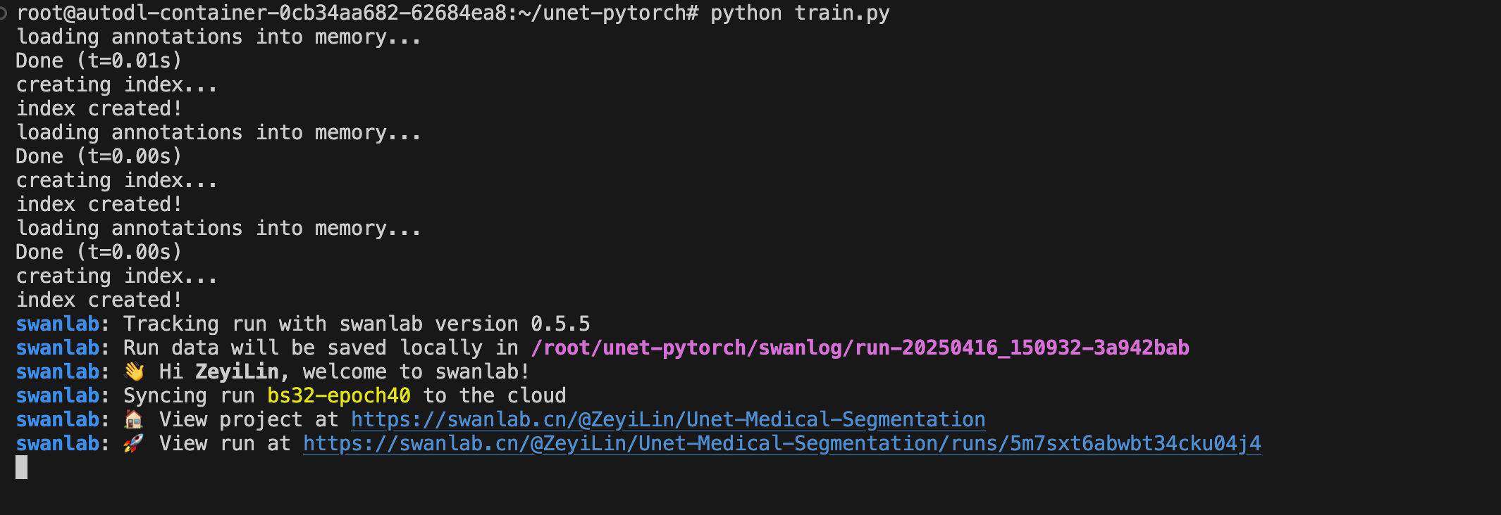
    main()

Run Training

python train.py

The following output indicates training has started:

6. Training Results

View detailed training progress here: Unet-Medical-Segmentation

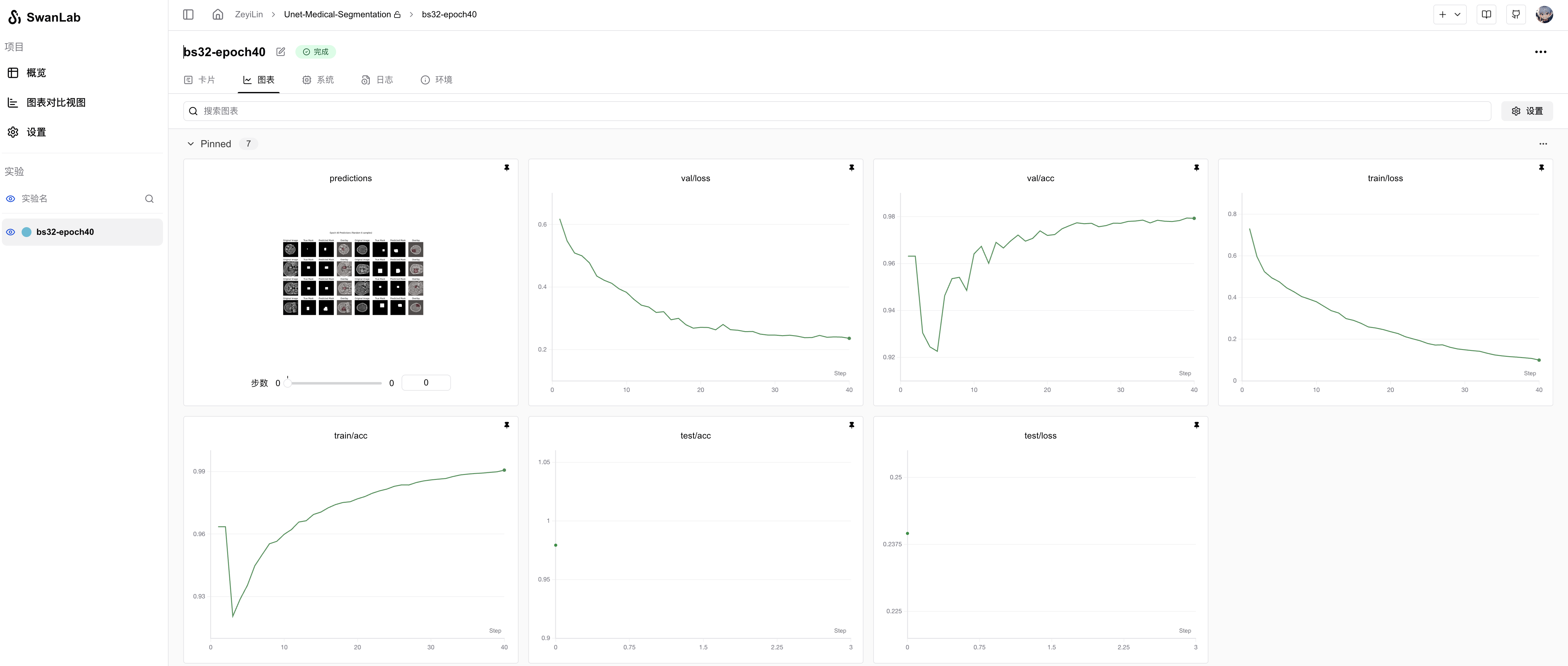
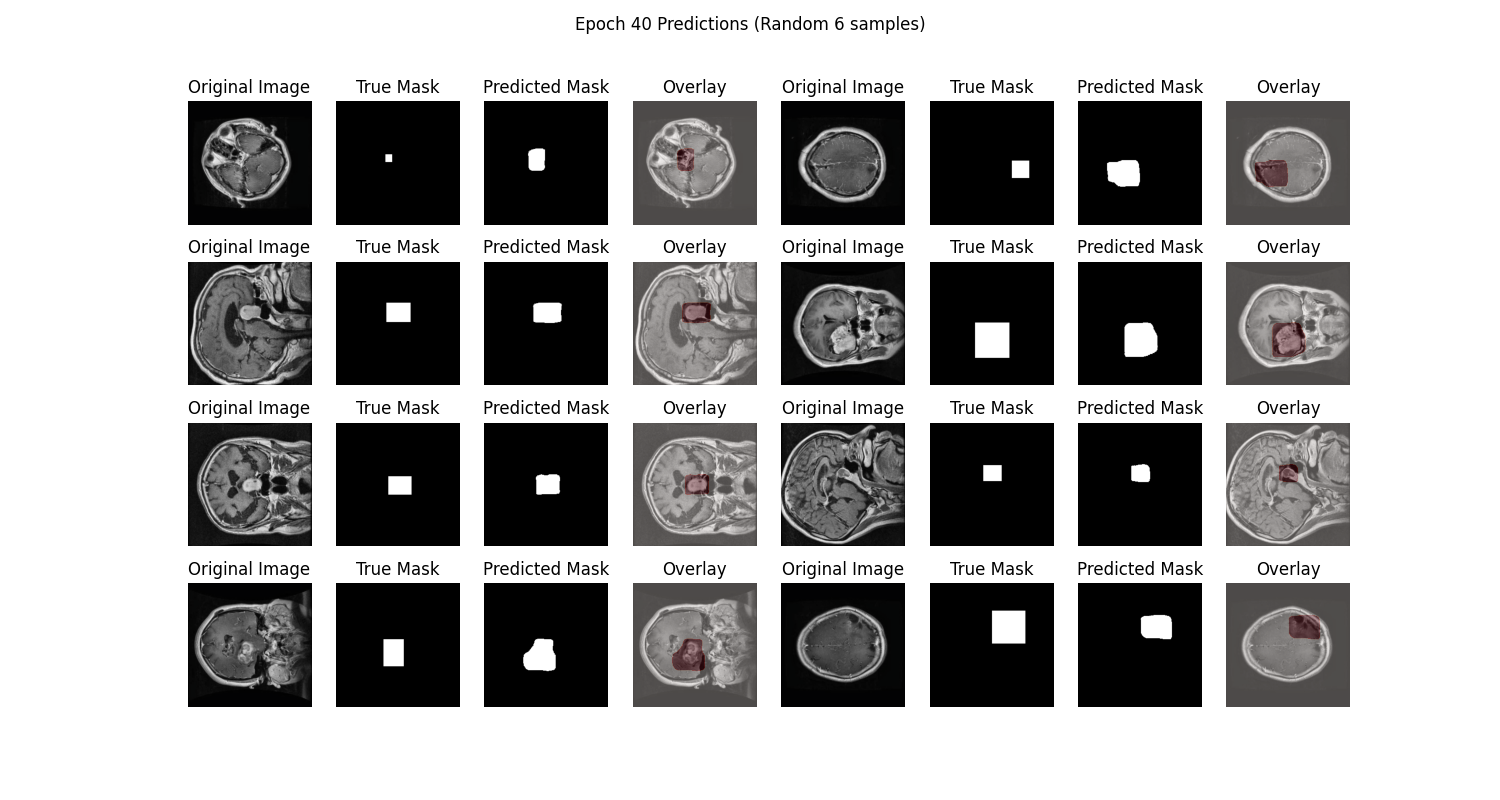
From the SwanLab charts, we observe that both training and validation losses decrease with epochs, while accuracies increase. The final test accuracy reaches 97.93%.

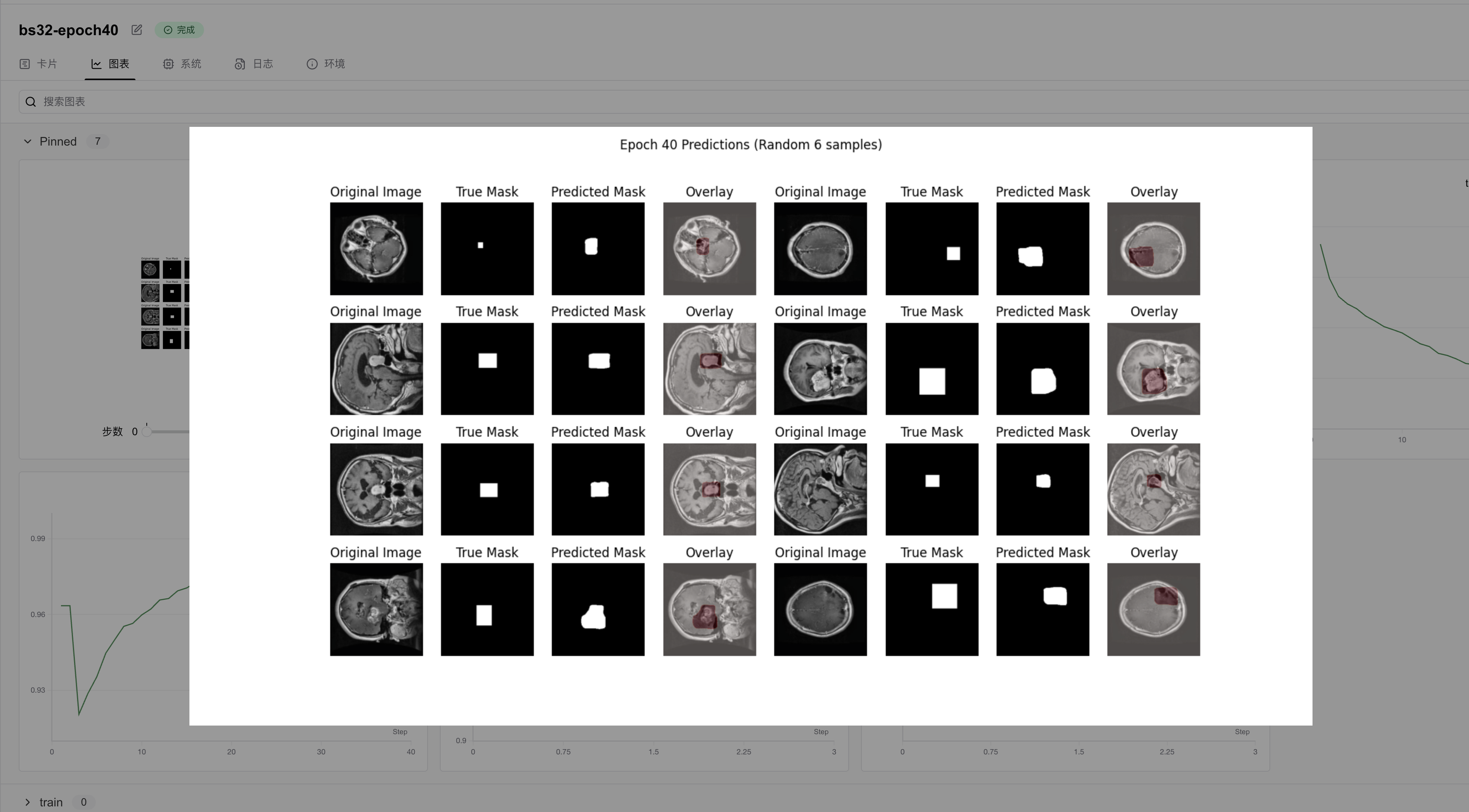
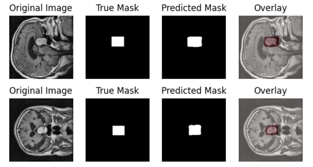
The prediction chart displays the model's segmentation results on the test set, showing relatively accurate tumor localization:

This tutorial primarily aims to introduce medical image segmentation training. For improved performance, consider experimenting with more complex architectures or data augmentation. Share your results on the SwanLab Benchmark Community!

7. Model Inference

Load the trained model (best_model.pth) and perform inference:

python predict.py

predict.py:

import torch
import torchvision.transforms as transforms
from PIL import Image
import matplotlib.pyplot as plt
from net import UNet
import numpy as np
import os

def load_model(model_path='best_model.pth', device='cuda'):
    """Load trained model"""
    try:
        # Check if file exists
        if not os.path.exists(model_path):
            raise FileNotFoundError(f"Model file not found at {model_path}")

        model = UNet(n_filters=32).to(device)
        state_dict = torch.load(model_path, map_location=device, weights_only=True)
        model.load_state_dict(state_dict)
        model.eval()
        print(f"Model loaded successfully from {model_path}")
        return model
    except Exception as e:
        print(f"Error loading model: {str(e)}")
        raise

def preprocess_image(image_path):
    """Preprocess input image"""
    image = Image.open(image_path).convert('RGB')
    display_image = image.resize((256, 256), Image.Resampling.BILINEAR)

    transform = transforms.Compose([
        transforms.ToTensor(),
        transforms.Resize((256, 256)),
        transforms.Normalize(mean=[0.485, 0.456, 0.406], std=[0.229, 0.224, 0.225])
    ])

    image_tensor = transform(image)
    return image_tensor.unsqueeze(0), display_image

def predict_mask(model, image_tensor, device='cuda', threshold=0.5):
    """Generate segmentation mask"""
    with torch.no_grad():
        image_tensor = image_tensor.to(device)
        prediction = model(image_tensor)
        prediction = (prediction > threshold).float()
    return prediction

def visualize_result(original_image, predicted_mask):
    """Visualize predictions"""
    plt.figure(figsize=(12, 6))
    plt.suptitle('Predictions')

    # Original image
    plt.subplot(131)
    plt.imshow(original_image)
    plt.title('Original Image')
    plt.axis('off')

    # Predicted mask
    plt.subplot(132)
    plt.imshow(predicted_mask.squeeze(), cmap='gray')
    plt.title('Predicted Mask')
    plt.axis('off')

    # Overlay
    plt.subplot(133)
    plt.imshow(np.array(original_image))
    plt.imshow(predicted_mask.squeeze(), cmap='Reds', alpha=0.3)
    plt.title('Overlay')
    plt.axis('off')

    plt.tight_layout()
    plt.savefig('./predictions.png')
    print("Visualization saved as predictions.png")

def main():
    device = torch.device("cuda" if torch.cuda.is_available() else "cpu")
    print(f"Using device: {device}")

    try:
        model_path = "./best_model.pth"
        print(f"Attempting to load model from: {model_path}")
        model = load_model(model_path, device)

        image_path = "dataset/test/27_jpg.rf.b2a2b9811786cc32a23c46c560f04d07.jpg"
        if not os.path.exists(image_path):
            raise FileNotFoundError(f"Image file not found at {image_path}")

        print(f"Processing image: {image_path}")
        image_tensor, original_image = preprocess_image(image_path)

        predicted_mask = predict_mask(model, image_tensor, device)
        predicted_mask = predicted_mask.cpu().numpy()

        print("Generating visualization...")
        visualize_result(original_image, predicted_mask)
        print("Results saved to predictions.png")

    except Exception as e:
        print(f"Error during prediction: {str(e)}")
        raise

if __name__ == '__main__':
    main()

Additional Notes

Hardware Specifications and Parameters

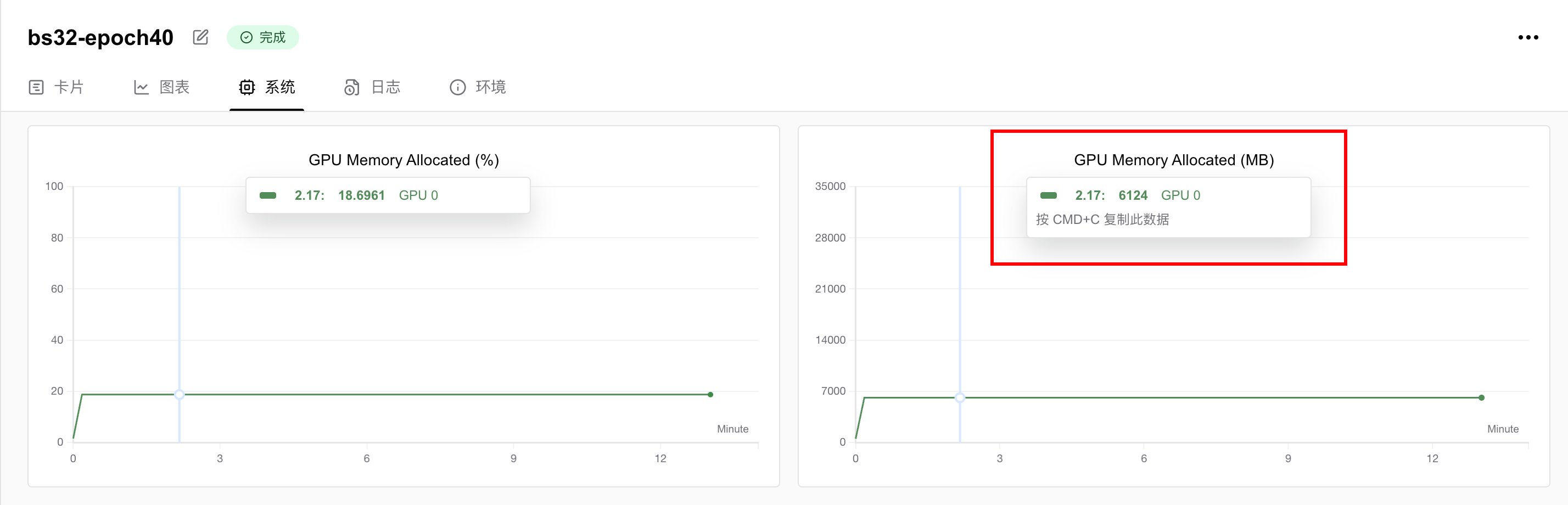
Training was conducted on an NVIDIA vGPU-32GB, completing 40 epochs in 13 minutes 22 seconds.

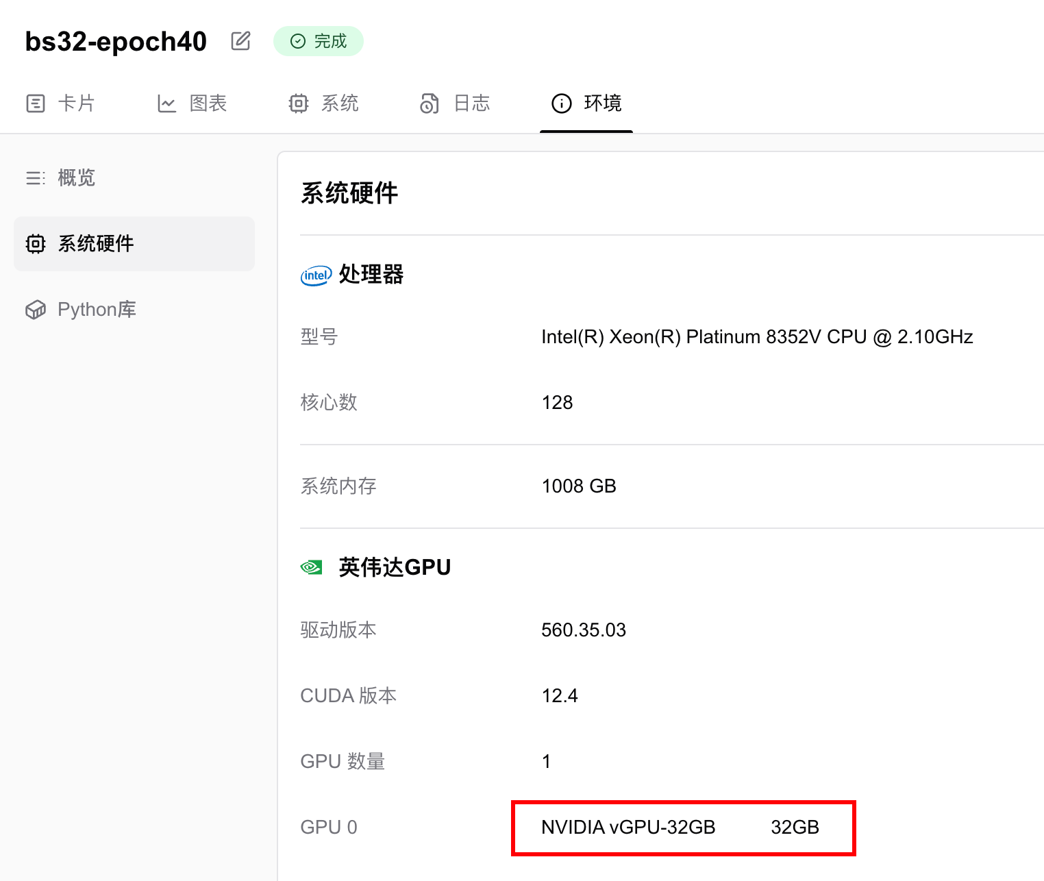
GPU memory usage was 6.124 GB, meaning any GPU with ≥6GB VRAM can run this task. To reduce memory requirements, decrease the batch size.

References

• Code: Full code in Section 5 or on GitHub
• Training Logs: Unet-Medical-Segmentation - SwanLab
• Model: UNet (PyTorch implementation)
• Dataset: brain-tumor-image-dataset-semantic-segmentation - Kaggle
• SwanLab: https://swanlab.cn